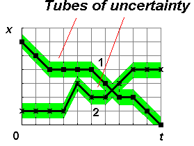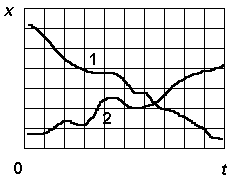
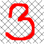
published in the Proceedings of the 3rd International Specialist Workshop on Nonlinear Dynamics of Electronic Systems (NDES-95), Dublin, Ireland, 28-29 July, 1995, pp. 249-252

APPLICATION OF CHAOTIC DYNAMICAL SYSTEMS TO THE PROBLEMS OF RECOGNITION AND CLASSIFICATION.

Yuri V. Andreyev, Alexander S. Dmitriev, Michael A. Matveyev

Institute of Radioengineering and Electronics
Russian Academy of Sciences
Moscow
RUSSIA

Abstract

In this report questions arising in attempts of application of nonlinear systems with complicated dynamics to image recognition are discussed, and approaches to their solution are proposed.

1 Introduction

Recognition problems are a real challenge to information processing systems. Even most important problems such as recognition of handwritten text or speech are solved only partially. This fact testifies to inefficiency of the approaches developed by far and prompts to search for new approaches, and among new candidates is a use of nonlinear dynamic systems.

In this report typical questions arising in attempts of application of nonlinear systems with complicated dynamics to image recognition are discussed, and approaches to their solution are proposed.

2 Compression of Information

A solution of a recognition problems needs compression of information related to images, and the compression must be irreversible.

Recognition needs information on the images. If the offered information is not irreversibly compressed, it means that we have full information on each image, and two images can be related to a certain class only if they completely coincide.


Two images from two different classes	Tubes of uncertainty represent compressed information

We can treat sets of features characteristic of the discussed images as the compressed information. To obtain a set of features for recognition we have to solve the problem of their extraction and their representativity. It is desirable for any recognition problem to have formal procedures allowing to create a system of representative features for the presented data.

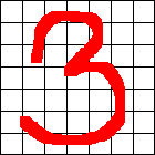
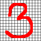
3 How Can We Plan Realization of These Formal Procedures?

Step 1. Original data related to each object is presented as a vector in a multidimensional space of features. To provide robustness of recognition procedure, the number of vectors is better be greater than the space dimension. The form of representation of the initial feature space seems not so important, it is important that its dimension be large enough.

Different forms of the initial feature space
Likewise, in the Takens procedure of restoring the pseudo-phase space it is also not important which component of the process (or their combination) is used, in principle, it has no effect on the result.

7x7 image transformed into a vector in a space of initial features
Step 2. Reduction of initial dimension of the vector describing an object with Karhunen-Loeve or similar method, i.e., calculation of covariance matrix, estimation of its eigenvalues, and projection of original data to a subspace of lower dimension (embedding space), based on eigenvectors.
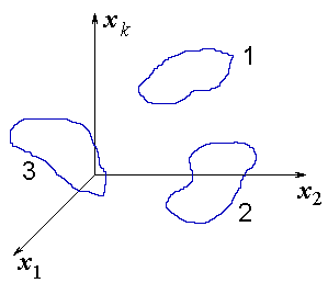
Step 3. Estimation of correlation dimension of the obtained reduced data set. If the correlation dimension is close to the embedding space dimension, then the problem cannot be further simplified. But there is indirect evidence that for a number of typical problems it is much lower [1, 2].

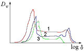4 Recognition With a Use of Correlation Dimension


Learning sets for image classes	Slopes of the correlation dimension for three different image classes

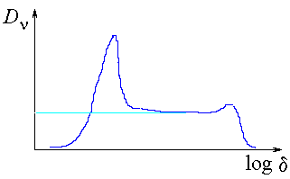
Recognition can be based on estimations of typical point dimension of a presented object from a class of recognized images. Of course, we calculate beforehand the correlation dimension for each class of images forming clusters in the embedding space.


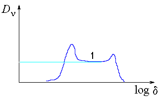Correlation integral slope for the images of class 1	Pointwise correlation integral slope for the images of class 1

5 Where Is Dynamics?

We can introduce dynamics in quite a number of ways.

(i) Synergetic computer by Haken [3].

It is used to process photographs. First, Fourier-images are obtained from original pictures (to provide tolerance to shifts). Then the dimension reduction is performed (step 2). A functional is made with local minima related to concrete images. When a new image is presented, it is used as initial conditions. A dynamical process is realized as a solution of the system of differential (or difference) equations evolving to one of the system equilibria.

(ii) Neural network by Hopfield [4].

Using such a net, one can work in the initial feature space. We can also reduce the space dimension using Karhunen-Loeve procedure. Dynamics appear here in solution of a system of differential equations evolving to one of the system equilibria, i.e., the situation is similar to synergetic computer. These two systems have another common feature: in both systems single objects , not classes of objects are recognized, because there is only a single specimen of each type of objects.

(iii) Feedforward neural networks with Back Propagation learning rule.

Using such networks one can work in the space of initial features, or in the embedding space. In the first case, information compression occurs through formation of the matrix of couplings. Dynamics is introduced at the stage of learning by tuning the couplings to minimize error function. When forming feedforward network for recognition, it is necessary to have a “surplus” of inner layers. Only in this case a smooth map function can be formed.

Unlike the synergetic computer and Hopfield neural network, the feedforward neural networks can be used as classifiers because they have no limitations on the number of objects related to the same class.

Note that the three above examples of the use of dynamics for recognition need considerable computational resources, which sets restrictions on the volume of information these systems can process.

(iv) One-dimensional and multi-dimensional maps [5-8].

Using 1-D piecewise-linear maps and their generalization to higher dimensions for storing scalar and vector information, we can work in the space of initial features, as well as in the embedding space. Dynamics appears in iteration of the maps, and the image carriers here are dynamic attractors: stable or unstable limit cycles, or strange attractors. In these systems the recognition problem can be solved, in the sense of the search for the reference image most close to the presented one.

An important feature of system (iv) compared to the first three systems is its high computational efficiency. Indeed, it allows processing of ~ 1-10 Mbytes of information by typical computers (personal computers and workstations), which is at least by two orders as high as for systems (i) - (iii).

6 Embedding Space and Parameters of Order

The components of the embedding space can be treated as parameters of order. Indeed, these components are a minimum set of variables allowing description of the main object properties, i.e., it satisfies the requirements for the parameters of order.

6.1 Parameters Of Order And Coding Information For Storing

In piecewise-linear maps with stored information the dynamic system dimension is fixed (e.g., equal to 1). So a question arises: how do we account (if we really do) for the difference in the number of initial features of an object and the number of its essential features? It may seem a paradox, but to a certain extent the model takes this into account through the length of cycles after coding (compression). Short cycles correspond to objects with a little number of essential features (parameters of order), while long practically incompressible cycles correspond to the objects requiring large number of features for description. That is, if an information block (or a set of blocks) corresponding to the description of the recognized object, has a distinct structure, and hence is well compressed by coding, then the cycle corresponds to an object that can be described with a little number of features (parameters of order). If the compression is null, e.g., the information block represents a random sequence (similar to turbulence), we have a case of a large number of freedom degrees. In this case the description in terms of parameters of order is impossible, and a full microscopic description is necessary.

6.2 Storing Information In Piecewise-Linear Maps And Correlation Integral

Let us consider the process of storing a time series or a monochrome picture by a limit cycle of 1-D (or multi-dimensional) dynamic system. Let N be the length of the initial alphabet, i.e., the number of the discrete signal amplitude or the picture brightness grades. N also defines the accuracy of variables = 1/N. It is easy to see that the storage level q defining consecutive q-fragments (substrings) of an initial information block corresponds to the dimension of the pseudo-phase space in the Takens procedure of reconstruction of attractor by a time series.

We use coding procedure each time when looking through the information block (string) we find a fragment of the length q at least twice in the string. In the method of correlation integral this is absolutely equivalent to a pair of pseudo-vectors separated by the distance less than . The relation between and is defined by the chosen metrics. For example, if

(1)

i.e., the distance is defined as the maximum difference of the corresponding pseudo-vectors’ components, then in a case of coinciding fragments the distance between pseudo-vectors is

< = 1/N. (2)

If at least a single component of pseudo-vectors x_p of x_l is different then this pair doesn’t get into the sum of the correlation integral. When searching for the number of the pairs of coinciding fragments of the length q, we find the number of vectors in the correlation integral with the distance less than . If we double now the number of quantization levels for the time series (or the number of brightness grades for the picture) for the fixed q, then the number of identical fragments m( /2) will be equal to the number of points in the correlation integral with the distance less than /2. Thus

m() ~ ^d, (3)

where d is the correlation dimension of the set of pseudo-vectors corresponding to the time series or the picture.

6.3 Attractor For “Recalling” Objects And Its Local Approximation

An object represented as a time series can be related to a trajectory in the pseudo-phase space. A set of objects belonging to some class can be also related to one or a few trajectories in the this space. These trajectories set a basis for a design of linear local predictor, that can be used for solution of recognition problems.

7 Linear And Nonlinear Predictors

Predictors are to predict further values of a system by a set of previous samples and are treated as dynamic systems imitating a real process.

Equations for a linear predictor are

(4)

where c_k are coefficients of linear prediction and are errors at i-th step.

Equations for a nonlinear predictor are

x_i+1 = f(x_i) + , (5)

where f is a nonlinear function of vector x_i = (x_i,x_i+1, ... ,x_i+d-1). In both cases d is the embedding space dimension. The embedding space dimension is determined from condition of a sharp decrease of prediction error with an increase in d.

Imagine now, that we design a linear and a nonlinear predictor for a chaotic signal born by a nonlinear dynamic system. Let for certainty the dynamic system be a quadratic map. Then a one-dimensional linear predictor will operate bad, because a linear system cannot produce chaotic signal. From the other hand, a one-dimensional nonlinear predictor (a local linear predictor can be used) will provide good prediction. What will happen if we dare to predict the behavior of the series generated by a two-dimensional nonlinear dynamic system with a one-dimensional local linear predictor? The prediction will be much worse, in general, than in the case of prediction of a one-dimensional dynamic system. The plot of x_n+1=g(x_n) will have sharp peaks and chasms. So to provide good prediction, the system x_n+1=g(x_n) must be smooth. Only in this case little changes in the initial conditions will not lead to drastic changes in the results.

7.1 Predictors With Storing Information In Piecewise-Linear Maps

Experiments on storing chaotic trajectories generated by logistic map (parabolic function) indicate that the resulting piecewise-linear map is close to parabola in a “rough” scale, but detailed examination shows a presence of “shelves”, i.e., inclined straight line segments, corresponding to information districts.

Storing information of general kind in 1-D map gives highly rugged map function. Hence direct application of informatively saturated low-dimensional piecewise-linear maps for prediction seems problematical. But one can try to use them in search for the nearest neighbors in linear local predictors.

7.2 Dynamic Systems And Image Recognition

The raggedness of the low-dimensional map function in which information is stored prevents realization of image recognition because of very small vicinity of attraction basins of attractors with the stored information. But if the embedding space is chosen for the stored data (e.g., by their preliminary coding) with dimension d, then the synthesized function will be substantially more smooth. This gives a good chance to a synthesis of a dynamical system in which the attractors bearing the stored information will have attraction basins corresponding to the objects of the same class as the attractor itself. In the vicinity of a reference cycle the dynamical system can look quite the same as in the initial method of storing information by stable limit cycles. But aside of it a construction of the kind of a local linear predictor is used.

7.3 Predictors And Synchronizators

After the stage of the design of the dynamic system generating information sequences close to the stored objects, it is necessary to introduce a mechanism of identification of a newly presented object to one of the classes represented in the dynamic system. The effect of chaotic synchronization realized in the systems with the stored information (synchronizators) can be used for this purpose.

Acknowledgments

This work is supported in part by a grant from the Russian Foundation for Fundamental Investigations (93-012-730) and by a NATO Linkage Grant (HT NATO LG No 930749).

References

[1] Yu. I. Neimark, Z. S. Batalova, Yu. G. Vasin, M. D. Breydo, Pattern Recognition And Medical Diagnostics, Nauka, Moscow, 1972 (in Russian).

[2] M. D. Alder, R. Togneri, Y. Attikiouzel, “Dimension Of The Speech Space”, IEE Proceedings-I, vol.138, No 3, pp.207-214, 1991.

[3] H. Haken, Information And Self-Organization. A Microscopic Approach To Complex Systems, Springer-Verlag, Berlin, 1988.

[4] J. J. Hopfield, “Neural Networks And Physical Systems With Emergent Collective Computation Abilities”, Proc. Natl. Acad. Sci. USA, vol.79, pp.2554-2558, 1982.

[5] A. S. Dmitriev, “Storing And Recognition Of Information In 1-D Dynamic Systems”, Radiotekhnika i Elektronika, vol.36, No 1, pp.101-108, 1991 (in Russian).

[6] A. S. Dmitriev, A. I. Panas, S. O. Starkov, “Storing And Recognition Information Based On Stable Cycles Of One-Dimensional Maps”, Phys. Lett. A, vol.155, No 8/9, pp.494-499, 1991.

[7] Yu. V. Andreyev, A. S. Dmitriev, L. O. Chua, C. W. Wu, “Associative And Random Access Memory Using 1-D Maps”, Int. Journal of Bifurcation and Chaos, vol.3, No 2, pp.483-504, 1992.

[8] Yu. V. Andreyev, Yu. L. Belsky, A. S. Dmitriev, “Storing And Retrieval Of Information Using Stable Cycles Of Two- And Multi-Dimensional Maps”, Radiotekhnika i Elektronika, vol.39, No 1, pp.114-123, 1994 (in Russian).